$$W(x, y) = \alpha \cdot \exp\left(-\frac{(x - x_0)^2 + (y - y_0)^2}{2\sigma^2}\right)$$
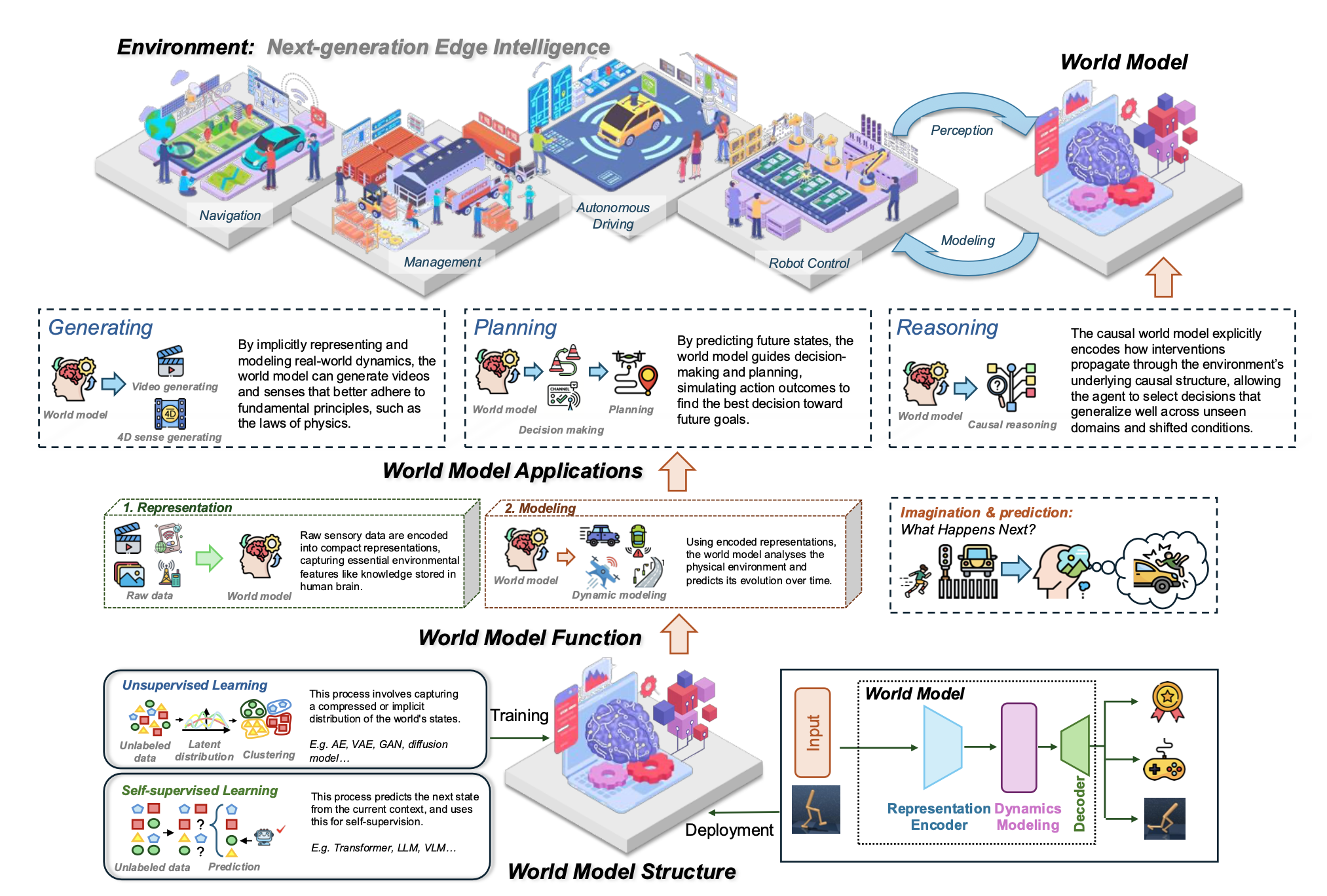
Illustration of world models for next-generation edge intelligence. The bottom part shows the workflow and structure of world models, including their training and deployment. The middle part illustrates the core functions of world models. The top part highlights the three core applications of world models and their potential application in a real-world environment.
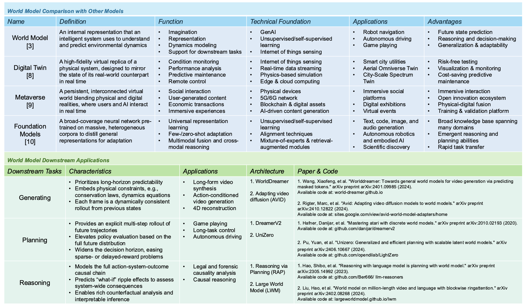
Comparison of World Models with Other Models and Their Downstream Applications
Tutorial: Wireless Dreamer for wireless edge intelligence optimization
Wireless Dreamer
We propose Wireless Dreamer, a novel world model-based reinforcement learning framework tailored for wireless edge intelligence optimization, particularly in low-altitude wireless networks (LAWNs). Furthermore, we present a case study on weather-aware UAV trajectory planning and demonstrate how the proposed framework leverages a world model to enhance wireless optimization.
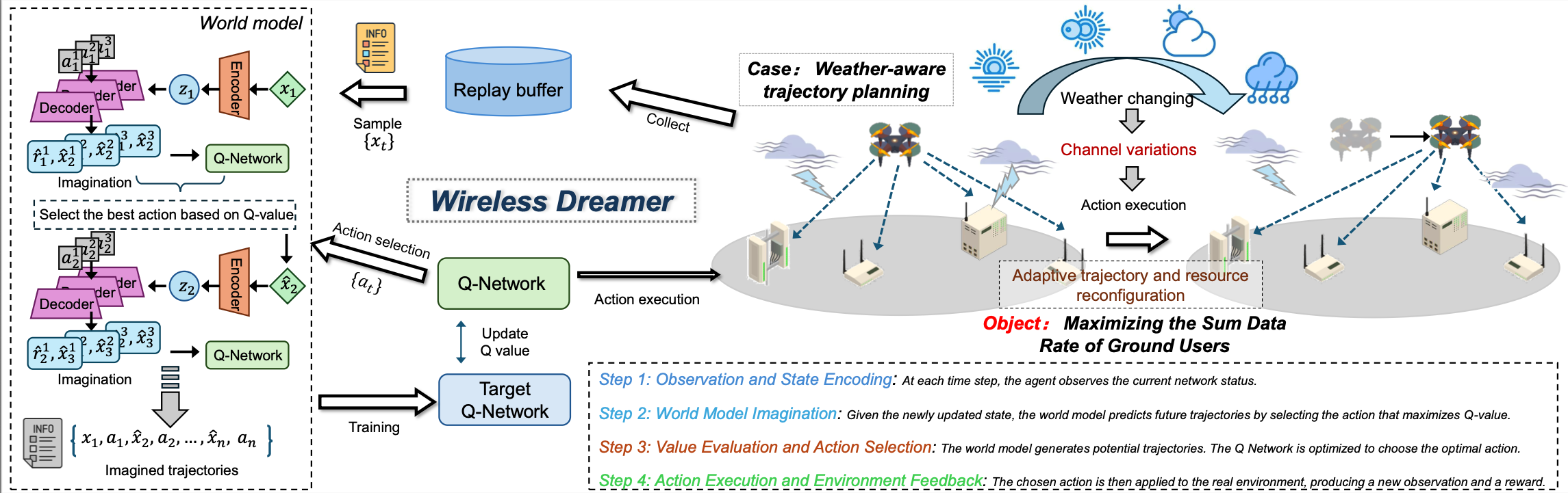
Figure 1: The workflow of the proposed framework. The left part is the model structure of Wireless Dreamer, including a world model, Q-network, and target Q-network. The bottom part presents the continuous processes of Wireless Dreamer. The right part illustrates the weather-aware tracking planning in a UAV-assisted scenario in LAWNs.
Weather-aware UAV trajectory planning
We consider a UAV-assisted wireless communication scenario in LAWNs, where a single UAV acts as a mobile base station to provide downlink coverage for multiple ground users under dynamic and spatially varying weather conditions, as shown in Figure 1. The UAV traverses a two-dimensional area over a fixed time horizon and dynamically adjusts its position to optimize communication performance while responding to evolving environmental factors such as wind intensity.
Weather-aware Environment Setup
The WeatherAwareUAVEnv is a Gym-compatible simulator for UAV-based wireless optimization in dynamic environments. It supports OFDMA channel modeling, energy constraints, and weather dynamics.
Key Parameters
- Grid Size: 64×64 (each cell is 4×4 meters)
- Users: 10 randomly placed ground users
- UAV Altitude: Fixed at 100 meters
- Bandwidth: 100 MHz at 28 GHz mmWave
- Action Space: 9 discrete movement directions (including no-op)
- Reward: Average per-user throughput in Mbps (optionally penalized by movement cost)
Weather Modeling
We adopt a drifting Gaussian hotspot to simulate dynamic weather disturbances. At each step, the storm center moves with drift and noise, generating a rainfall map:
- \( \alpha \): intensity (default 0.7)
- \( (x_0, y_0) \): storm center (drifts over time)
- \( \sigma \): Gaussian width proportional to grid size
Path Loss under Weather
Weather intensity affects path loss as follows:
$$PL(d) = PL_0 + 10 \cdot n \cdot \log_{10}(d) + \beta \cdot W(x, y)$$
- \( PL_0 \): base loss (e.g., 60 dB)
- \( n \): exponent (e.g., 2.5)
- \( \beta \): sensitivity to weather (e.g., 10)
Environment Parameters
- \( \text{grid\_size} \): 64 (Grid dimensions: 64 × 64)
- \( N_{\text{users}} \): 10 (Number of ground users)
- \( T_{\max} \): 100 steps (Maximum steps per episode)
- \( h_{\text{UAV}} \): 100 m (UAV altitude)
- \( \Delta_{\text{cell}} \): 4 m (Grid cell size)
- \( K_{\text{OFDMA}} \): 64 (OFDMA subcarriers)
- \( R_{\text{threshold}} \): 10 Mbps (Coverage threshold)
Weather Model
Weather intensity map follows a Gaussian distribution with drift:
$$W(x, y, t) = I_W \cdot \exp\left(-\frac{(x - c_x(t))^2 + (y - c_y(t))^2}{2\sigma^2}\right)$$
- \( I_W \): Weather intensity = 0.7
- \( (c_x(t), c_y(t)) \): Weather center position at time \( t \)
- \( \sigma \): Weather spread = grid_size / 5.0 ≈ 12.8
- \( v_{\text{drift}} \): Drift speed = (0.3, 0.2) grid cells/step
- \( \sigma_{\text{noise}} \): Gaussian noise = 0.2
DQN Network Parameters
Q-value update (TD learning):
$$\mathcal{L}_Q = \mathbb{E}_{(s,a,r,s')\sim\mathcal{D}}\left[\left(r + \gamma \max_{a'}Q_{\text{target}}(s',a') - Q(s,a)\right)^2\right]$$
Epsilon decay:
$$\epsilon_{t+1} = \max(\epsilon_{\min}, \lambda_{\epsilon} \cdot \epsilon_t)$$
- \( \alpha_Q \): 1e-3 (Q-network learning rate)
- \( \gamma \): 0.99 (Discount factor)
- \( \epsilon_{\text{start}} \): 1.0 (Initial epsilon for exploration)
- \( \epsilon_{\text{min}} \): 0.1 (Minimum epsilon)
- \( \lambda_{\epsilon} \): 0.995 (Epsilon decay rate)
- \( f_{\text{target}} \): 10 episodes (Target network update frequency)
- \( d_{\text{hidden}} \): 128 (Hidden layer dimension)
World Model (Transition Model) Parameters
State encoding:
$$h_s = \text{MLP}_{\text{encoder}}(s) \in \mathbb{R}^{16}$$
Combined features:
$$z = [h_s; \text{one-hot}(a)] \in \mathbb{R}^{25}$$
(16-dim encoded state + 9-dim one-hot action)
Next state and reward prediction:
$$\hat{s}' = \text{MLP}_{\text{state}}(z)$$
$$\hat{r} = \text{MLP}_{\text{reward}}(z)$$
World model loss:
$$\mathcal{L}_M = \mathbb{E}_{(s,a,r,s')\sim\mathcal{D}}\left[\|s' - \hat{s}'\|^2 + |r - \hat{r}|^2\right]$$
- \( \alpha_M \): 1e-3 (World model learning rate)
- \( d_{\text{encoder}} \): 16 (State encoder output dimension)
- \( d_{\text{hidden}} \): 128 (Hidden layer dimension)
- \( f_{\text{model}} \): 4 episodes (Model update frequency)
- \( \rho_{\text{model}} \): 0.7 (Model-generated data ratio)
- \( K_{\text{rollout}} \): 5 steps (Rollout steps for synthetic data)
Model-Based Planning Parameters
Planning objective (when enabled):
$$a^* = \arg\max_{a_0} \sum_{i=1}^{N_{\text{samples}}} \sum_{t=0}^{H_{\text{plan}}} \gamma^t \hat{r}_t(s_t, a_t^{(i)})$$
- \( H_{\text{plan}} \): 5 steps (Planning horizon)
- \( N_{\text{samples}} \): 10 (Number of action sequences sampled)
- \( \text{use\_planning} \): True (Planning disabled by default)
Experience Replay Parameters
- \( C_{\text{buffer}} \): 16,000 (Replay buffer capacity)
- \( B \): 64 (Batch size for training)
Experimental Setup
Our experiment is based on Python along with the PyTorch package, conducted on a Linux server equipped with an Ubuntu 22.04 operating system and powered by an Intel(R) Xeon(R) Silver 4410Y 12-core processor and an NVIDIA RTX A6000 GPU. We benchmark the proposed method with DQN and random policy.
Results
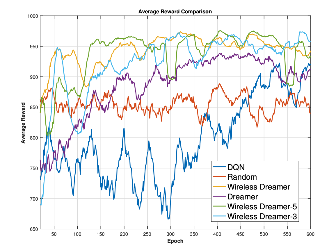
Figure 2: Comparison of average episodic rewards
Results
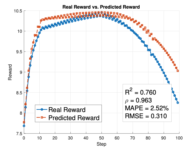
Figure 3: Comparison between real and predicted rewards
The experimental results demonstrate the effectiveness of Wireless Dreamer in improving learning efficiency and decision quality.
BibTeX
@article{zhao2025world,
  title={World Models for Cognitive Agents: Transforming Edge Intelligence in Future Networks},
  author={Zhao, Changyuan and Zhang, Ruichen and Wang, Jiacheng and Zhao, Gaosheng and Niyato, Dusit and Sun, Geng and Mao, Shiwen and Kim, Dong In},
  journal={arXiv preprint arXiv:2506.00417},
  year={2025}
}